本文共 9839 字，大约阅读时间需要 32 分钟。

Tensorflow揭秘

 

 

 

为了理解新的Tensorflow框架--Google的机器学习计算平台，通过一个玩具级的例子来学习它。

 

下面就是Google介绍这个框架的描述：

TensorFlow™ 是一个采用数据流图（data flow graphs），用于数值计算的开源软件库。节点（Nodes）在图中表示数学操作，图中的线（edges）则表示在节点间相互联系的多维数据数组，即张量（tensor）。它灵活的架构让你可以在多种平台上展开计算，例如台式计算机中的一个或多个CPU（或GPU），服务器，移动设备等等。TensorFlow 最初由Google大脑小组（隶属于Google机器智能研究机构）的研究员和工程师们开发出来，用于机器学习和深度神经网络方面的研究，但这个系统的通用性使其也可广泛用于其他计算领域。

 

What goes on within machine learning code is math, it helps to organize this in a way that simplifies and keeps the computative flow organized.

 

张量（Tensors）

首先遇到的第一个问题就是：张量是什么东西？它是怎么样流动呢？

一个向量（vector）是一串值的列表，一个矩阵（matrix）是一个数表（或者列表的列表）...，从而产生了一个数表的列表（或者列表的列表的列表），或者一个数表的数表（矩阵的矩阵），依次类推。所有数值使用张量表示，在机器学习里的任何等式都可以发现张量的存在。

 

现在让我们从一个已经学习过的例子来学习多层神经网络。

在这个例子里，我们使用数据特征值(‘x1’, ‘x2’, …)流过两层的神经网络、以及每个节点（神经元）、每个权重值(‘W’)和偏差值（‘b’)，最后输出y值。

 

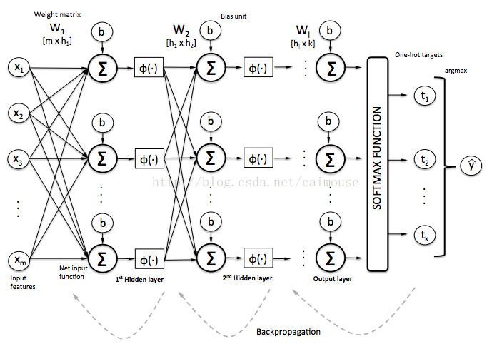
从上图可以看到，从输入值（‘X’）到输出值（‘Y’），经历了一系列（flow）数字流的计算（math），在数学计算上，使用了多维的矩阵（张量），常量和变量（比如b1）。定义和执行这些数字流的计算，这就是TensorFlow框架所做的事情。

 

 

由于通过这些数字流的计算，为了与预期的输出达到一致，必须不断地调整权重值和偏差值，从而让这个模型建立起来。TF框架平台提供了在GPU上加速计算的能力，这对于大规模数据训练时就特别有用。除此之外，TF框架也提供了很多数学公式的计算，这样对于开发和编写代码就特别方便了。这也就是为什么使用框架平台的原因。

 

在TensorFlow的学习里，最经典的开始教程就是直接识别手写数字或鸢尾花卉数据集（）（或者在其它机器学习的框架也是如此）。当然使用这些实质性的数据来学习是比较有用的，但是这些数据对于一个机器学习新手来说，还是一个比较复杂的事情，所以这里采用一些玩具级别的数据来给新手学习。

 

For training data to achieve ‘toy’ status the data itself should be intuitive and easily grasped.

玩具级的数据集

让我们来构造一个只有5个元素的数组，让它当作输入。输出更简单，只有[0,1]或[1,0]两个，这两个输出的结果依赖于这个数组的第1位和最后1位是否为打开（也即是1）：

[0, 1, 1, 1, 1], [0,1]

[1, 1, 1, 1, 0], [0,1]

[1, 1, 1, 0, 0], [0,1]

[1, 1, 0, 0, 0], [0,1]

[1, 0, 0, 0, 1], [1,0]

[1, 1, 0, 0, 1], [1,0]

[1, 1, 1, 0, 1], [1,0]

[1, 0, 0, 1, 1], [1,0]

 

仔细地看一下上面的数据集，就可以凭直感知道输入与输出的关系，从而建立一个模型。

 

如果我们使用这些数据来训练机器学习的模型，然后再使用它来预测5个元素的数组，是否可以呢？它是否预测正确吗？这就是一个机器学习的问题，具体的定义：软件学习模式。

 

代码

下面将要使用TensorFlow来建立一个模型，并且定义这些数据集，然后训练这个模型，再让它做一些预测。代码在这里：

 

下面的代码就是基本的库导入，如下：

import numpy as npimport randomimport tensorflow as tf

接着定义数据：

def create_feature_sets_and_labels(test_size = 0.3):    # known patterns (5 features) output of [1] of positions [0,4]==1    features = []    features.append([[0, 0, 0, 0, 0], [0,1]])    features.append([[0, 0, 0, 0, 1], [0,1]])    features.append([[0, 0, 0, 1, 1], [0,1]])    features.append([[0, 0, 1, 1, 1], [0,1]])    features.append([[0, 1, 1, 1, 1], [0,1]])    features.append([[1, 1, 1, 1, 0], [0,1]])    features.append([[1, 1, 1, 0, 0], [0,1]])    features.append([[1, 1, 0, 0, 0], [0,1]])    features.append([[1, 0, 0, 0, 0], [0,1]])    features.append([[1, 0, 0, 1, 0], [0,1]])    features.append([[1, 0, 1, 1, 0], [0,1]])    features.append([[1, 1, 0, 1, 0], [0,1]])    features.append([[0, 1, 0, 1, 1], [0,1]])    features.append([[0, 0, 1, 0, 1], [0,1]])    features.append([[1, 0, 1, 1, 1], [1,0]])    features.append([[1, 1, 0, 1, 1], [1,0]])    features.append([[1, 0, 1, 0, 1], [1,0]])    features.append([[1, 0, 0, 0, 1], [1,0]])    features.append([[1, 1, 0, 0, 1], [1,0]])    features.append([[1, 1, 1, 0, 1], [1,0]])    features.append([[1, 1, 1, 1, 1], [1,0]])    features.append([[1, 0, 0, 1, 1], [1,0]])    # shuffle out features and turn into np.array    random.shuffle(features)    features = np.array(features)    # split a portion of the features into tests    testing_size = int(test_size*len(features))    # create train and test lists    train_x = list(features[:,0][:-testing_size])    train_y = list(features[:,1][:-testing_size])    test_x = list(features[:,0][-testing_size:])    test_y = list(features[:,1][-testing_size:])    return train_x, train_y, test_x, test_y

在上面这段代码里，把三分之二的数据拿来训练模型，三分之一的数据拿来测试。这个比率的设置是通过变量test_size来定义的，并且通过随机函数shuffle来随机抽取一部分数据来执行，这样每次拿到的数据并不是一样的，通过这些数据不断实验和反复迭代。

 

现在可以使用TensorFlow来建立模型：

train_x, train_y, test_x, test_y = create_feature_sets_and_labels()# hidden layers and their nodesn_nodes_hl1 = 20n_nodes_hl2 = 20# classes in our outputn_classes = 2# iterations and batch-size to build out modelhm_epochs = 1000batch_size = 4    x = tf.placeholder('float')y = tf.placeholder('float')# random weights and bias for our layershidden_1_layer = {'f_fum':n_nodes_hl1,                  'weight':tf.Variable(tf.random_normal([len(train_x[0]), n_nodes_hl1])),                  'bias':tf.Variable(tf.random_normal([n_nodes_hl1]))}hidden_2_layer = {'f_fum':n_nodes_hl2,                  'weight':tf.Variable(tf.random_normal([n_nodes_hl1, n_nodes_hl2])),                  'bias':tf.Variable(tf.random_normal([n_nodes_hl2]))}output_layer = {'f_fum':None,                'weight':tf.Variable(tf.random_normal([n_nodes_hl2, n_classes])),                'bias':tf.Variable(tf.random_normal([n_classes])),}

上面建立了模型，共使用了20个节点和2层隐藏层，并使用随机值来初始化这些权重值和偏差值，同时也定义了输出层。

我们现在可以对这个模型来建立数学的等式关系了：

# our predictive model's definitiondef neural_network_model(data):    # hidden layer 1: (data * W) + b    l1 = tf.add(tf.matmul(data,hidden_1_layer['weight']), hidden_1_layer['bias'])    l1 = tf.sigmoid(l1)    # hidden layer 2: (hidden_layer_1 * W) + b    l2 = tf.add(tf.matmul(l1,hidden_2_layer['weight']), hidden_2_layer['bias'])    l2 = tf.sigmoid(l2)    # output: (hidden_layer_2 * W) + b    output = tf.matmul(l2,output_layer['weight']) + output_layer['bias']    return output

请认真地查看这段代码，并且与前面神经网络图进行比较，在这里我们使用矩阵的乘法（tf.matmul），矩阵（张量）、权重值、偏差，并且定义激活函数tf.sigmoid，这些函数都是TF框架提供机器学习的内置API函数。

# hidden layer 1: (data * W) + b

l1 = tf.add(tf.matmul(data,hidden_1_layer[‘weight’]), hidden_1_layer[‘bias’]) l1 = tf.sigmoid(l1)

上面的代码跟前面学习过两层神经网络是一样的，但是现在使用TF框架来简化代码的编写，计算过程也被封装起来了。仔细地查看神经网络图，比较之前的代码和现在TF编写的代码，你应该发现它们其实是相等的。矩阵的乘法就更加简单了。

 

There’s no black-magic here: math is math.

现在开始来训练上面建立好的模型：

# training our modeldef train_neural_network(x):    # use the model definition    prediction = neural_network_model(x)    # formula for cost (error)    cost = tf.reduce_mean( tf.nn.softmax_cross_entropy_with_logits(prediction,y) )    # optimize for cost using GradientDescent    optimizer = tf.train.GradientDescentOptimizer(1).minimize(cost)    # Tensorflow session    with tf.Session() as sess:        # initialize our variables        sess.run(tf.global_variables_initializer())        # loop through specified number of iterations        for epoch in range(hm_epochs):            epoch_loss = 0            i=0            # handle batch sized chunks of training data            while i < len(train_x):                start = i                end = i+batch_size                batch_x = np.array(train_x[start:end])                batch_y = np.array(train_y[start:end])                _, c = sess.run([optimizer, cost], feed_dict={x: batch_x, y: batch_y})                epoch_loss += c                i+=batch_size                last_cost = c            # print cost updates along the way            if (epoch% (hm_epochs/5)) == 0:                print('Epoch', epoch, 'completed out of',hm_epochs,'cost:', last_cost)                # print accuracy of our model        correct = tf.equal(tf.argmax(prediction, 1), tf.argmax(y, 1))        accuracy = tf.reduce_mean(tf.cast(correct, 'float'))        print('Accuracy:',accuracy.eval({x:test_x, y:test_y}))        # print predictions using our model        for i,t in enumerate(test_x):            print ('prediction for:', test_x[i])            output = prediction.eval(feed_dict = {x: [test_x[i]]})            # normalize the prediction values            print(tf.sigmoid(output[0][0]).eval(), tf.sigmoid(output[0][1]).eval())        train_neural_network(x)

如果你把这段代码与之前没有使用框架的代码进行比较，发现它们竟然是相同的，训练的过程没有任何的变化。当我们通过周期地训练这个模型，让它的错误（损失函数）越来越来少，就把这个模型训练好了。

现在让我们查看一下它的输出和训练过程的信息：

Epoch   0 completed out of 1000 cost: 1.06944

Epoch 200 completed out of 1000 cost: 0.000669607

Epoch 400 completed out of 1000 cost: 0.00030982

Epoch 600 completed out of 1000 cost: 0.00019792

Epoch 800 completed out of 1000 cost: 0.00014411

Accuracy: 1.0

prediction for: [1, 1, 1, 1, 1]

0.998426 0.392255

prediction for: [1, 0, 1, 1, 1]

0.99867 0.364066

prediction for: [0, 0, 1, 1, 1]

0.028218 0.997783

prediction for: [0, 1, 0, 1, 1]

0.0528865 0.997093

prediction for: [1, 0, 0, 0, 1]

0.999507 0.413642

prediction for: [1, 0, 0, 1, 0]

0.0507428 0.998406

注意到这里，当训练超过1000次之后，它的错误将会减少。这里计算精度的数据是采用测试数据，而不是采用训练的数据。

接着下来，我们就可以使用它来预测测试数据了。当输入[1, _, _, _, 1]的形式时，它输出[1,0]；当输入其它模式时，就输出[0,1]。每个值输出来时概率值：

prediction for: [1, 0, 0, 1, 0]

0.0507428 0.998406

这里就意味着模型已经认为输入的模式与[1, _, _, _, 1]模式有严重的不同。

在这里采用玩具级的数据来解释，可以让你的精力主要放在代码上面，而不数据集。这个两层的神经网络ANN的工作方式，你立即可以借鉴它，使用它去对鸢尾花分类，或者去预测股票的市场走势了。

 

训练代码详细介绍

让我们再回过头来看一下训练代码，我们定义了变量prediction等于训练的模型：

# use the model definition

 prediction = neural_network_model(x)

接着告诉TF框架怎么样来优化这个模型：

c = tf.reduce_mean(tf.nn.softmax_cross_entropy_with_logits(prediction,y))

 optimizer = tf.train.GradientDescentOptimizer(1).minimize(c)

当然我们也可以使用TF框架其它的优化方法来建立这个模型。

接着下来，通过周期地迭代这个模型:

with tf.Session() as sess:

 sess.run(tf.global_variables_initializer())

for epoch in range(hm_epochs):

 _, c = sess.run([optimizer, cost], feed_dict={x: batch_x, y: batch_y})

通过每一小批次数据的训练，这个模型每一次就调整它的权重值和偏差值（朝它减少错误的方向进行）。

这个模型的精度计算是采用测试数据来评估的：

correct = tf.equal(tf.argmax(prediction, 1), tf.argmax(y, 1))

accuracy = tf.reduce_mean(tf.cast(correct, ‘float’))

print(‘Accuracy:’,accuracy.eval({x:test_x, y:test_y}))

最后使用这个模型来处理一些新数据的结果，就非常简单了，它直接使用激活函数来计算输出值0和1：

print (‘prediction for:’, test_x)

output = prediction.eval(feed_dict = {x: [test_x]})

print(tf.sigmoid(output[0][0]).eval(), tf.sigmoid(output[0][1]).eval())

 

整个过程是怎么样呢

我们通过机器学习算法来实现识别5个数字数组的预测模式，它是通过训练数据来实现的：

提供[1, _, _, _, 1] 和其它数据。它是通过查看这些数据来学习，并没有人为地告诉它怎么样预测这些数组。与传统的编程模式进行比较，就是像下面这样:

def identify_pattern(data):

    if data[0]==1 and data[-1]==1:

        return [1,0]

    else:

        return [0,1]

    

print(test_x[0], identify_pattern(test_x[0]))

显然上面这个过程就不是机器学习了，它是采用人为制定的规则来进行解决问题。如果我们采用写规则这种方式来编写程序处理图像识别的问题，就会遇到非常大的困难。到这里，我们应该理解这些预测模型，其实就是通过一些数据，或者说数字流的方式来通过这些计算等式来形成的。

现在，你可以有经验来学习处理更真实的问题了，比如手写数字的识别。

1. TensorFlow API攻略

3. C++标准模板库从入门到精通 

4.跟老菜鸟学C++

5. 跟老菜鸟学python

6. 在VC2015里学会使用tinyxml库

7. 在Windows下SVN的版本管理与实战